Graphical Independence Networks

A vignette for the gRain package

Søren Højsgaard

Bayesian networks

Introduction

The gRain package implements Bayesian Networks (hereafter often abbreviated BNs). The name gRain is an acronym for [gra]phical [i]ndependence [n]etworks. The main reference for gRain is Højsgaard (2012), see also citation("gRain").

Moreover, Højsgaard, Edwards, and Lauritzen (2012) gives a broad treatment of graphical models (including Bayesian networks) More information about the package, other graphical modelling packages and development versions is available from

Example: Chest clinic

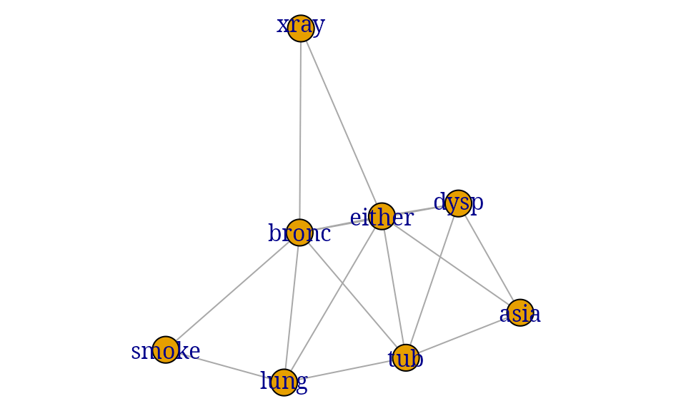
This section reviews the chest clinic example of Lauritzen and Spiegelhalter (1988) (illustrated in Figure @ref(fig:chest-LS)) and shows one way of specifying the model in gRain. Lauritzen and Spiegelhalter (1988) motivate the chest clinic example with the following narrative:

``Shortness–of–breath (dyspnoea) may be due to tuberculosis, lung cancer or bronchitis, or none of them, or more than one of them. A recent visit to Asia increases the chances of tuberculosis, while smoking is known to be a risk factor for both lung cancer and bronchitis. The results of a single chest X–ray do not discriminate between lung cancer and tuberculosis, as neither does the presence or absence of dyspnoea.’’

chest_dag <- dag(list("asia", c("tub", "asia"), "smoke", c("lung", "smoke"), c("bronc", 
"smoke"), c("either", "tub", "lung"), c("xray", "either"), c("dysp", 
"bronc", "either")))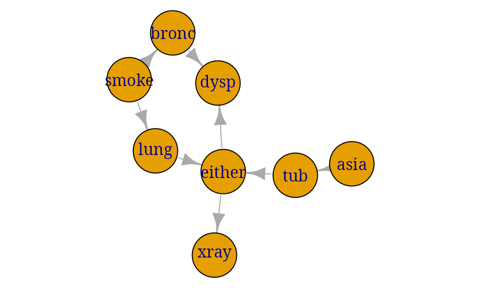

Chest clinic example from Lauritzen and Spiegelhalter (1988).

Building a Bayesian network

The description above involves the following binary variables: $a=\mbox{asia}$, $s=\mbox{smoker}$, $t=\mbox{tuberculosis}$, $l=\mbox{lung cancer}$, $b=\mbox{bronchitis}$, $e=\mbox{either tuberculosis or lung cancer}$, $d=\mbox{dyspnoea}$ and $x=\mbox{xray}$.

Each variable is binary and can take the values “yes” and “no”: Note that $e$ is a logical variable which is true (yes) if either $t$ or $l$ are true (yes) and false (no) otherwise. The connection between the variables is displayed by the DAG (directed acyclic graph) in Figure~@ref(fig:chest-LS).

A joint probability density factorizing according to a DAG with nodes $V$ can be constructed as follows: Each node $v\in V$ has a set $pa(v)$ of parents and each node $v\in V$ has a finite set of states. A joint distribution over the variables $V$ can be given as a product of conditional distributions

$$\begin{align} (\#eq:dagfact1) p(V) = \prod_{v\in V} p(v|pa(v)) \end{align}$$

where $p(v|pa(v))$ is a function defined on $(v,pa(v))$. This function satisfies that $$\sum_{v^*} p(v=v^*|pa(v))=1,$$

i.e. that for each configuration of the parents $pa(v)$, the sum over the levels of $v$ equals one. Hence $p(v|pa(v))$ becomes the conditional distribution of $v$ given $pa(v)$. In practice $p(v|pa(v))$ is specified as a table called a conditional probability table or a CPT for short. Thus, a Bayesian network can be regarded as a complex stochastic model built up by putting together simple components (conditional probability distributions). A joint probability density for all eight variables in Figure~@ref(fig:chest-LS) can be constructed as

$$\begin{align} (\#eq:chestfact1) p(V) = p(a)p(s)p(t|a)p(l|s)p(b|s)p(e|t,l) p(d|e, b)p(x|e). \end{align}$$

Queries to networks

Suppose we are given the evidence (sometimes also called “finding”) that a set of variables $E\subset V$ have a specific value $e^*$. With this evidence, we are often interested in the conditional distribution $p(v|E=e^*)$ for some of the variables $v \in V \setminus E$ or in $p(U|E=e^*)$ for a set $U\subset V \setminus E$. Interest might also be in calculating the probability of a specific event, e.g. the probability of seeing a specific evidence, i.e. $p(E=e^*)$. Other types of evidence (called soft evidence, virtual evidence or likelihood evidence) are discussed in Section @ref(sec:hard-soft).

For example that a person has recently visited Asia and suffers from dyspnoea, i.e. $a=\mbox{yes}$ and $d=\mbox{yes}$. In the chest clinic example, interest might be in $p(l|e^*)$, $p(t|e^*)$ and $p(b|e^*)$, or possibly in the joint (conditional) distribution $p(l,t,b|e^*)$.

A one–minute version of gRain

Specifying a Bayesian network

A simple way of specifying the model for the chest clinic example is as follows.

Specify conditional probability tables (with values as given in Lauritzen and Spiegelhalter (1988)) (there are other ways of specifying conditional probability tables, see the package documentation):

yn <- c("yes","no")
a    <- cpt(~asia, values=c(1, 99),levels=yn)
t.a  <- cpt(~tub|asia, values=c(5, 95, 1, 99),levels=yn)
s    <- cpt(~smoke, values=c(5, 5), levels=yn)
l.s  <- cpt(~lung|smoke, values=c(1, 9, 1, 99), levels=yn)
b.s  <- cpt(~bronc|smoke, values=c(6, 4, 3, 7), levels=yn)
e.lt <- cpt(~either|lung:tub,values=c(1, 0, 1, 0, 1, 0, 0, 1),levels=yn)
x.e  <- cpt(~xray|either, values=c(98, 2, 5, 95), levels=yn)
d.be <- cpt(~dysp|bronc:either, values=c(9, 1, 7, 3, 8, 2, 1, 9), levels=yn)

Compile list of conditional probability tables.

chest_cpt <- compile_cpt(a, t.a, s, l.s, b.s, e.lt, x.e, d.be)
chest_cpt

##  P( asia )
##  P( tub | asia )
##  P( smoke )
##  P( lung | smoke )
##  P( bronc | smoke )
##  P( either | lung tub )
##  P( xray | either )
##  P( dysp | bronc either )

The components are arrays, but coercion into dataframes sometimes makes it easier to digest the components.

chest_cpt$tub

##      asia
## tub    yes   no
##   yes 0.05 0.01
##   no  0.95 0.99

chest_cpt$tub  |> as.data.frame.table()

##   tub asia Freq
## 1 yes  yes 0.05
## 2  no  yes 0.95
## 3 yes   no 0.01
## 4  no   no 0.99

Create the network:

chest_bn <- grain(chest_cpt)
chest_bn

## Independence network: Compiled: TRUE Propagated: FALSE Evidence: FALSE

Default is that the network is compiled at creation time, but if one chooses not to do so, compilation can be done with:

chest_bn <- compile(chest_bn)

Setting evidence and querying a network

In the chest clinic example, there are three disease variables, two background variables and two symptoms. Following the narrative, we can set evidence that a person has recently visited Asia and has dyspnoea:

disease <- c("tub", "lung", "bronc")
asia_dysp <- list(asia="yes", dysp="yes")

Initially, the network can be queried without evidence:

chest_bn |> querygrain(nodes=disease, type="marginal")

## $tub
## tub
##    yes     no 
## 0.0104 0.9896 
## 
## $lung
## lung
##   yes    no 
## 0.055 0.945 
## 
## $bronc
## bronc
##  yes   no 
## 0.45 0.55

chest_bn |> querygrain(nodes=disease, type="marginal", simplify = TRUE)

##          yes     no
## tub   0.0104 0.9896
## lung  0.0550 0.9450
## bronc 0.4500 0.5500

chest_bn |> querygrain(nodes=disease, type="joint") 

## , , bronc = yes
## 
##      lung
## tub         yes       no
##   yes 0.0003276 0.004352
##   no  0.0311724 0.414148
## 
## , , bronc = no
## 
##      lung
## tub         yes       no
##   yes 0.0002444 0.005476
##   no  0.0232556 0.521024

chest_bn |> querygrain(nodes=disease, type="joint", simplify = TRUE)

##   tub lung bronc      Freq
## 1 yes  yes   yes 0.0003276
## 2  no  yes   yes 0.0311724
## 3 yes   no   yes 0.0043524
## 4  no   no   yes 0.4141476
## 5 yes  yes    no 0.0002444
## 6  no  yes    no 0.0232556
## 7 yes   no    no 0.0054756
## 8  no   no    no 0.5210244

chest_bn |> querygrain(nodes=disease, type="conditional")

## , , bronc = yes
## 
##      lung
## tub      yes     no
##   yes 0.0104 0.0104
##   no  0.9896 0.9896
## 
## , , bronc = no
## 
##      lung
## tub      yes     no
##   yes 0.0104 0.0104
##   no  0.9896 0.9896

chest_bn |> querygrain(nodes=disease, type="conditional", simplify = TRUE)

##   tub lung bronc   Freq
## 1 yes  yes   yes 0.0104
## 2  no  yes   yes 0.9896
## 3 yes   no   yes 0.0104
## 4  no   no   yes 0.9896
## 5 yes  yes    no 0.0104
## 6  no  yes    no 0.9896
## 7 yes   no    no 0.0104
## 8  no   no    no 0.9896

Above we obtain the marginal, joint distributions and conditional distribution for the disease variables. The output can in some cases be simplified to dataframes. For the conditional distribution, we obtain the conditional distribution of the first node given the rest of the nodes.

Setting evidence

Evidence can be entered in different ways:

asia_dysp <- list(asia="yes", dysp="yes")

chest_ev <- chest_bn |>
    evidence_add(evidence=asia_dysp)

The evidence is a list and can conveniently be displayed as a dataframe:

chest_ev |> evidence_get() 

##   nodes is_hard hard_state evi_weight
## 1  asia    TRUE        yes       1, 0
## 2  dysp    TRUE        yes       1, 0

chest_ev |> querygrain(nodes=disease, simplify = TRUE)

##           yes     no
## tub   0.08775 0.9122
## lung  0.09953 0.9005
## bronc 0.81140 0.1886

chest_ev |> evidence_prob()

## [1] 0.004501

The network can be queried again, and we can also obtain the probability of observing this evidence:

chest_ev |> querygrain(nodes=disease, simplify=TRUE)

##           yes     no
## tub   0.08775 0.9122
## lung  0.09953 0.9005
## bronc 0.81140 0.1886

chest_ev |> evidence_prob()

## [1] 0.004501

chest_bn |> evidence_prob(evidence=list(asia="yes", dysp="yes"))

## [1] 0.004501

The probability of observing a specific evidence can be found by setting the evidence as a vector of weights. This is useful in connection with soft evidence (also called likelihood evidence), see Section~@ref(sec:hard-soft).

Hints and shortcuts

An alternative way of specifying a network is by first defining CPTs and then entering values afterwards. Programmatically, this can be done as:

yn <- c("yes", "no")

node_parents_list <-
    list("asia", c("tub", "asia"), "smoke", c("lung", "smoke"),
         c("bronc", "smoke"), c("either", "tub", "lung"),
         c("xray", "either"), c("dysp", "bronc", "either"))

chest_dummy_cpt2 <- lapply(node_parents_list, function(f){
    cpt(f, levels=yn)
})
bn_temp <- compile_cpt(chest_dummy_cpt2) |> grain()

Above the network has ones in all potentials. Next update values in (some of the) potentials:

cpt_values <- list(asia=c(1, 99),
                   tub=c(5, 95, 1, 99),
                   smoke=c(5, 5),
                   lung=c(1, 9, 1, 99),            
                   bronc=c(6, 4, 3, 7),
                   either=c(1, 0, 1, 0, 1, 0, 0, 1),
                   xray=c(98, 2, 5, 95),
                   dysp=c(9, 1, 7, 3, 8, 2, 1, 9))
bn_real <- replace_cpt(bn_temp, cpt_values)

bn_temp |> querygrain(evi=asia_dysp, nodes=disease, simplify = TRUE)

##       yes  no
## tub   0.5 0.5
## lung  0.5 0.5
## bronc 0.5 0.5

bn_real |> querygrain(evi=asia_dysp, nodes=disease, simplify = TRUE)

##           yes     no
## tub   0.08775 0.9122
## lung  0.09953 0.9005
## bronc 0.81140 0.1886

Consider querying a network where focus is on marginal distributions (the default). If all variables have the same levels (as the case is here), the output can be coerced to a dataframe:

querygrain(chest_bn, nodes=disease, simplify = TRUE)

##          yes     no
## tub   0.0104 0.9896
## lung  0.0550 0.9450
## bronc 0.4500 0.5500

In the more general case the output can be coerced to a list of dataframes

querygrain(chest_bn, nodes=disease, result="data.frame")

## $tub
## tub
##    yes     no 
## 0.0104 0.9896 
## 
## $lung
## lung
##   yes    no 
## 0.055 0.945 
## 
## $bronc
## bronc
##  yes   no 
## 0.45 0.55

A typical use of gRain involves setting evidence and then querying the network afterwards. This can all be done in one call of querygrain() (notice that this does not alter the network object):

chest_bn |> querygrain(evidence=asia_dysp,
                       nodes=disease, simplify = TRUE)

##           yes     no
## tub   0.08775 0.9122
## lung  0.09953 0.9005
## bronc 0.81140 0.1886

Evidence can be also be given as a vector of weights.

chest_bn |> querygrain(evidence=list(asia=c(1, 0), dysp=c(1, 0)),
                       nodes=disease, simplify = TRUE)

##           yes     no
## tub   0.08775 0.9122
## lung  0.09953 0.9005
## bronc 0.81140 0.1886

The weights must be non-negative but need not sum to one. This is important in connection with soft evidence (also called likelihood evidence), see Section~@ref(sec:hard-soft). Above, the weights could also have been set as c(.1, 0). The important part is that the zero excludes certain states as being impossible.

Nodes on which evidence is given are not reported unless exclude=FALSE

querygrain(chest_bn,
           evidence=list(asia=c(1, 0), dysp=c(1, 0)),
           nodes=c("lung", "bronc", "asia", "dysp"),
           exclude=FALSE, simplify = TRUE)

##           yes     no
## asia  1.00000 0.0000
## lung  0.09953 0.9005
## bronc 0.81140 0.1886
## dysp  1.00000 0.0000

If nodesare not specified, queries for all nodes without evidence are reported.

querygrain(chest_bn,
           evidence=asia_dysp,
           simplify = TRUE)

##            yes     no
## tub    0.08775 0.9122
## lung   0.09953 0.9005
## either 0.18230 0.8177
## bronc  0.81140 0.1886
## smoke  0.62592 0.3741
## xray   0.21954 0.7805

If nodes are not specified and exclude=FALSE, then queries for all nodes are reported.

querygrain(chest_bn,
           evidence=asia_dysp,
           exclude = FALSE, simplify = TRUE)

##            yes     no
## asia   1.00000 0.0000
## tub    0.08775 0.9122
## lung   0.09953 0.9005
## either 0.18230 0.8177
## bronc  0.81140 0.1886
## smoke  0.62592 0.3741
## dysp   1.00000 0.0000
## xray   0.21954 0.7805

Conditioning on evidence with zero probability

Consider setting the evidence

chest_bn3 <- evidence_add(chest_bn, evidence=list(either="no", tub="yes"))

Under the model, this specific evidence has zero probability: either is true if tub is true or lung is true (or both). Hence the specific evidence is impossible and therefore, all conditional probabilities are (under the model) undefined:

evidence_prob(chest_bn3)

## [1] 0

querygrain(chest_bn3, nodes=disease, type="joint")

##      bronc
## lung  yes  no
##   yes NaN NaN
##   no  NaN NaN

Hard and soft (likelihood) evidence

Below we describe how to work with virtual evidence (also known as soft evidence or likelihood evidence) in gRain. This is done via the function evidence_add().

The clique potential representation in a Bayesian network gives $$\begin{align} p(x) \propto \psi(x) = \prod_{C} \psi_C(x_C). \end{align}$$

Here we recall that the whole idea in computations with Bayesian networks is to avoid calculation the product on the right hand side above. Instead computations are based on propagation (multiplying, dividing and summing clique potentials $\psi_C$ in an appropriate order, and such an appropriate order comes from a junction tree). The normalizing constant, say $c=\sum_x \psi(x)$, comes out of propagation as a “by-product”.

Suppose a set of nodes $E$ are known to have a specific value, i.e. $x_E=x^*_E$. This is called hard evidence. The probability of the event $x_E=x^*_E$ is $$\begin{align} p(x_E=x^*_E)=E_p\{I(x_E=x^*_E)\} = \sum_x I(x_E=x^*_E) p(x) = \frac{1}{c} \sum_x I(x_E=x^*_E) \psi(x) \end{align}$$

The computations are based on modifying the clique potentials $\psi_C$ by giving value zero to states in $\psi_C$ which are not consistent with $x_E=x^*_E$. This can be achieved with an indicator function, say $L_C(x_C)$ such that we obtain a set of new potentials $\tilde \psi_C(x) = L_C(x_C) \psi_C(x_C)$. Propagation with these new potentials gives, as a by product, $\tilde c=\sum \tilde \psi(x)$ where $\tilde\psi(x)= \prod_C \tilde\psi_C(x_C)$. Consequently, we have $p(x_E=x^*_E)=\tilde c / c$.

In a more general setting we may have non–negative weights $L(x)$ for each value of $x$. We may calculate $$\begin{align} E_p\{L(X)\} = \sum_x L(x)p(x) \end{align}$$ If $L(X)$ factorizes as $L(X)= \prod_C L_C(X_C)$ then the computations are carried out as outlined above, i.e. by the message passing scheme.

Hard evidence

Suppose we want to make a diagnosis about tuberculosis given the evidence that a person is a smoker. We call such evidence hard evidence because the state of the variables are known with certainty. The function setEvidence() can be used for this purpose. The following forms are equivalent (the reason will be explained below):

chest_ev1 <- chest_bn |> evidence_add(list(smoke="yes"))
chest_ev2 <- chest_bn |> evidence_add(list(smoke=c(1, 0)))

chest_bn |> querygrain(nodes=disease, simplify = TRUE)

##          yes     no
## tub   0.0104 0.9896
## lung  0.0550 0.9450
## bronc 0.4500 0.5500

chest_ev1 |> querygrain(nodes=disease, simplify = TRUE)

##          yes     no
## tub   0.0104 0.9896
## lung  0.1000 0.9000
## bronc 0.6000 0.4000

Soft evidence (also called virtual evidence or likelihood evidence)

Suppose we are not certain if a patient is a smoker or not. We shall assume that for patients who are smokers, we would (correctly) guess so in 80% of the cases, whereas for patients who are not smokers we would (erroneously) guess that they are smokers in 10% of the cases.

In gRain this, situation can be handled in two different ways. One way is to introduce a new variable smoke_guess with smoke as its only parent and then we enter evidence for this node.

g.s <- cpt(~ smoke_guess|smoke, levels=yn,
              values=c(.8, .2, .1, .9))
g.s

##            smoke
## smoke_guess yes  no
##         yes 0.8 0.1
##         no  0.2 0.9

chest_ext <- c(cpt_list, list(g.s)) |> compile_cpt() |> grain()
chest_ext |> querygrain(nodes=disease, simplify = TRUE)

##          yes     no
## tub   0.0104 0.9896
## lung  0.0550 0.9450
## bronc 0.4500 0.5500

chest_ext |> querygrain(nodes=disease, evidence=list(smoke="yes"), simplify = TRUE)

##          yes     no
## tub   0.0104 0.9896
## lung  0.1000 0.9000
## bronc 0.6000 0.4000

chest_ext |> querygrain(nodes=disease, evidence=list(smoke_guess="yes"), simplify = TRUE)

##          yes     no
## tub   0.0104 0.9896
## lung  0.0900 0.9100
## bronc 0.5667 0.4333

Another approach is to enter virtual evidence in the original network as shown below.

chest_ve <- chest_bn |>
    evidence_add(evidence = list(smoke = c(.8, .1)))
chest_ve |> querygrain(nodes=disease, simplify = TRUE)

##          yes     no
## tub   0.0104 0.9896
## lung  0.0900 0.9100
## bronc 0.5667 0.4333

evidence_get(chest_ve)

##   nodes is_hard hard_state evi_weight
## 1 smoke   FALSE         NA   0.8, 0.1

Consequently, specifying the hard evidence that smoke="yes" can be done as

chest_bn |> setEvidence(evidence=list(smoke=c(1, 0)))

## Independence network: Compiled: TRUE Propagated: TRUE Evidence: TRUE

Building a network from data

When building a network from data, there are two situations to be distinguished between. 1) The network is known and the data is used to estimate the parameters in the network. 2) The network is unknown and the data is used to estimate the network structure and the parameters in the network.

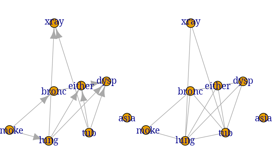
In both cases it is possible to have a network specified as a dag or as an undirected (chordal) graph. The following code illustrates how to build a network from data. The data is simulated data from the chest clinic example.

Building a network from a known network

The following list defines a dag for the chest clinic example: Each component is a list with two elements: the first element is the node and the second element is a vector of parents.

node_parents_list <- list("asia", c("tub", "asia"), "smoke", c("lung", "smoke"),
              c("bronc", "smoke"), c("either", "tub", "lung"),
              c("xray", "either"), c("dysp", "bronc", "either"))

g1 <- dag(node_parents_list)
par(mar=c(0,0,0,0))
plot(g1)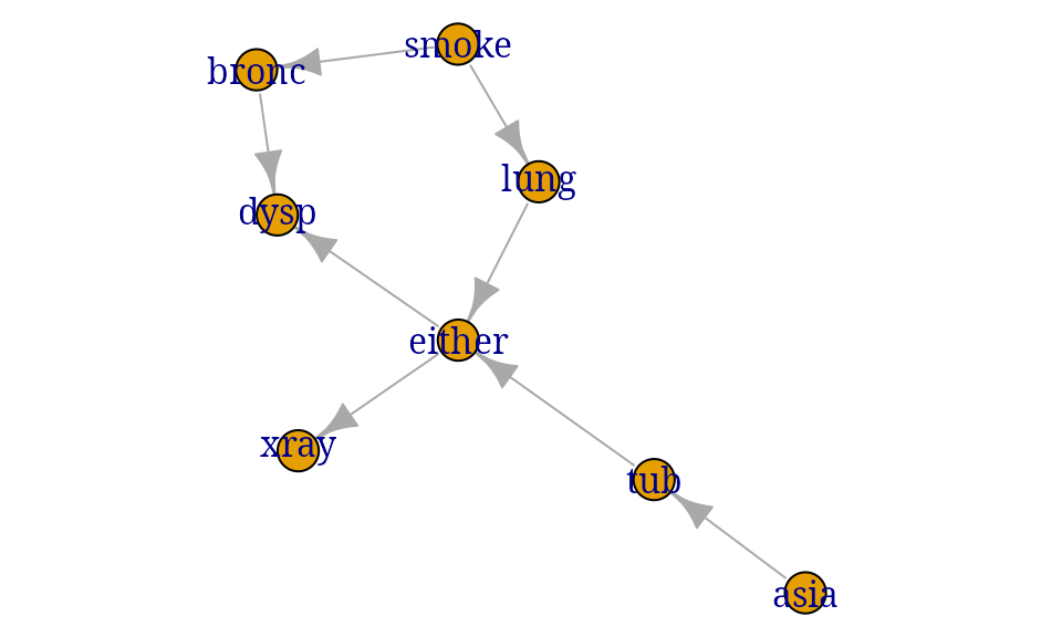

The following list defines an undirected graph for the chest clinic example: Each component is a list with the nodes in the clique.

cliq <- list(c("xray", "either"), c("asia", "tub"), c("smoke", "lung", 
"bronc"), c("lung", "either", "tub"), c("lung", "either", "bronc"
), c("bronc", "either", "dysp"))

g2 <- ug(cliq)
par(mar=c(0,0,0,0))
plot(g2)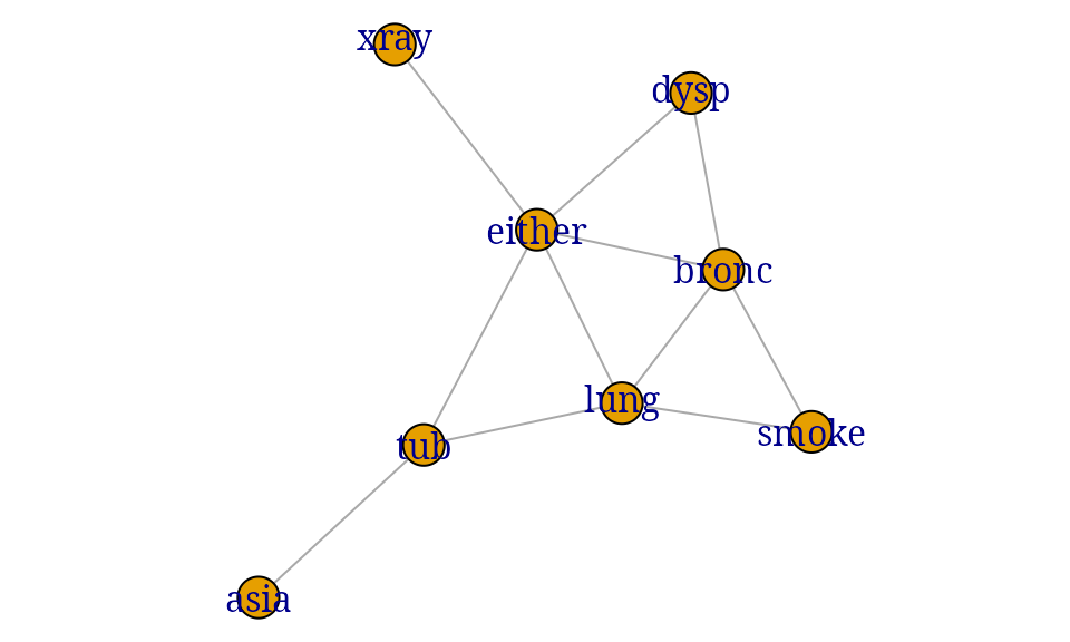

A netowrk can be built from data using:

bn1 <- grain(g1, data=gRbase::chestSim100000)
bn2 <- grain(g2, data=gRbase::chestSim100000)

## NAs found in clique potential(s) for clique(s): 
## c("bronc", "lung", "either") 
##   ... consider using the smooth argument

It is explained in the references that the two networks specify the same joint distribution because internally a dag is converted to an undirected chordal graph which provides the basis for the computations. In practice the two joint distributions differ slightly, and this is because the way in which information is extracted from data, see examples below.

j1 <- querygrain(bn1, type="joint")
j2 <- querygrain(bn2, type="joint")
d <- j1 %a-% j2
max(abs(d))

## [1] NaN

Building networks from data

The following two graphs specify the same model stating that A and C are conditionally independent given B. The first graph is a directed acyclic graph (DAG) and the second graph is an undirected graph (UG).

g1  <- dag(~A:C + B:C, result="igraph")
g2  <- ug(~A:C + B:C, result="igraph")
par(mfrow=c(1,2), mar=c(0,0,0,0))
plot(g1); plot(g2)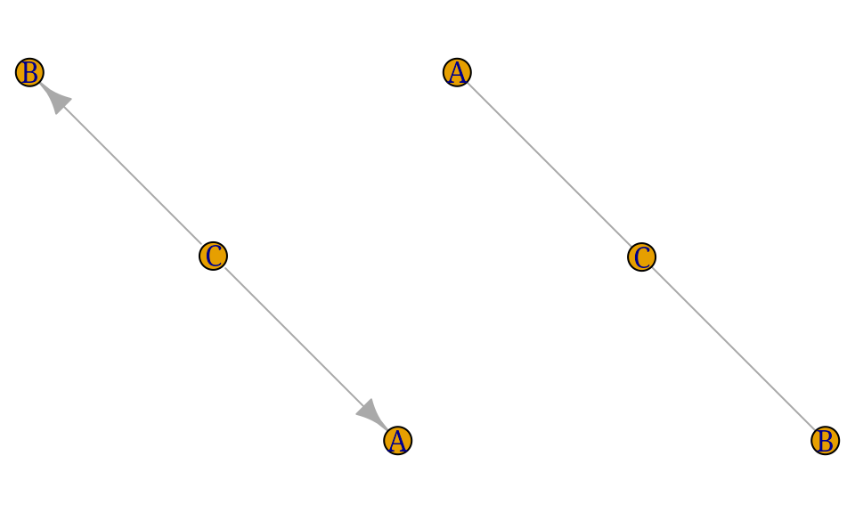

Given such a graph, we can build a network from data. Suppose data is as follows:

tab <- tabNew(~A:B:C, levels=c("+", "-"), 
              values=c(1, 2, 3, 5, 1, 2, 1, 4))

A network can be built from data using:

bn1 <- grain(g1, data=tab)
bn2 <- grain(g2, data=tab)

The two networks specify the same joint distribution:

j1 <- querygrain(bn1, type="joint")
j2 <- querygrain(bn2, type="joint")
d <- j1 %a-% j2
max(abs(d))

## [1] 2.776e-17

In the process of creating networks, conditional probability tables are extracted when the graph is a dag and clique potentials are extracted when the graph is a chordal (i.e. triangulated) undirected graph. This takes place as follows (internally):

Neet to estimate $p(A|B)$, $p(C|B)$ and $p(B)$ from the data. This can be done as follows:

p <- extract_cpt(tab, g1) |> c()
p

## [[1]]
## C
##      +      - 
## 0.5789 0.4211 
## 
## [[2]]
##    C
## A        +    -
##   + 0.3636 0.25
##   - 0.6364 0.75
## 
## [[3]]
##    C
## B        +     -
##   + 0.2727 0.375
##   - 0.7273 0.625

Likewise, we can extract the clique potentials from the data, call these $q(AC)$ and $q(BC)$:

q <- extract_pot(tab, g2) |> c()
q

## [[1]]
##    C
## A        +      -
##   + 0.2105 0.1053
##   - 0.3684 0.3158
## 
## [[2]]
##    C
## B        +     -
##   + 0.2727 0.375
##   - 0.7273 0.625

Clique potentials are not uniquely defined, but the product of clique potentials is. In the implementation in gRain, $q(AC)$ is the relative frequency in the $AC$-marginal table, i.e. $p(AB)$. Moreover and $q(BC)$ is the frequency in the $BC$-marginal table divided by the frequency in the $C$-marginal table. Hence, the product of the clique potentials and the product of the cpts is the same as the joint distribution:

tabProd(p) |> ftable()

##     C       +       -
## A B                  
## + +   0.05742 0.03947
##   -   0.15311 0.06579
## - +   0.10048 0.11842
##   -   0.26794 0.19737

tabProd(q) |> ftable()

##     C       +       -
## A B                  
## + +   0.05742 0.03947
##   -   0.15311 0.06579
## - +   0.10048 0.11842
##   -   0.26794 0.19737

Handling zeros in the data

Next suppose data is as follows

tab0 <- tab
tab0[1:4] <- 0
tab0

## , , C = +
## 
##    B
## A   + -
##   + 0 0
##   - 0 0
## 
## , , C = -
## 
##    B
## A   + -
##   + 1 1
##   - 2 4

In the process of creating networks above, the following quantities are computed:

n_BC <- tab0 |> tabMarg(~B:C)
n_AC <- tab0 |> tabMarg(~A:C)
n_C  <- tab0 |> tabMarg(~C)

p.B_C <- n_BC %a/% n_C
p.A_C <- n_AC %a/% n_C
p.C <- n_C / sum(n_C)
p.C

## C
## + - 
## 0 1

p.B_C

##    C
## B     +     -
##   + NaN 0.375
##   - NaN 0.625

p.A_C

##    C
## A     +    -
##   + NaN 0.25
##   - NaN 0.75

bn01 <- grain(g1, data=tab0)

## NAs found in cpt(s) for node(s): A, B
##   ... consider using the smooth argument

bn02 <- grain(g2, data=tab0)

## NAs found in clique potential(s) for clique(s): 
## c("B", "C") 
##   ... consider using the smooth argument

p <- extract_cpt(tab0, g1) |> c()

## NAs found in cpt(s) for node(s): A, B
##   ... consider using the smooth argument

q <- extract_pot(tab0, g2) |> c()

## NAs found in clique potential(s) for clique(s): 
## c("B", "C") 
##   ... consider using the smooth argument

p

## [[1]]
## C
## + - 
## 0 1 
## 
## [[2]]
##    C
## A     +    -
##   + NaN 0.25
##   - NaN 0.75
## 
## [[3]]
##    C
## B     +     -
##   + NaN 0.375
##   - NaN 0.625

q

## [[1]]
##    C
## A   +    -
##   + 0 0.25
##   - 0 0.75
## 
## [[2]]
##    C
## B     +     -
##   + NaN 0.375
##   - NaN 0.625

tabProd(p) |> ftable()

##     C       +       -
## A B                  
## + +       NaN 0.09375
##   -       NaN 0.15625
## - +       NaN 0.28125
##   -       NaN 0.46875

tabProd(q) |> ftable()

##     C       +       -
## A B                  
## + +       NaN 0.09375
##   -       NaN 0.15625
## - +       NaN 0.28125
##   -       NaN 0.46875

eps <- 0.01
bn01e <- grain(g1, data=tab0, smooth=eps)
bn02e <- grain(g2, data=tab0, smooth=eps)

j1 <- querygrain(bn01e, type="joint")
j2 <- querygrain(bn02e, type="joint")
j1

## , , B = +
## 
##    A
## C           +         -
##   + 0.0006219 0.0006219
##   - 0.0941379 0.2805496
## 
## , , B = -
## 
##    A
## C           +         -
##   + 0.0006219 0.0006219
##   - 0.1564809 0.4663440

j2

## , , B = +
## 
##    C
## A           +       -
##   + 0.0006219 0.09383
##   - 0.0006219 0.28055
## 
## , , B = -
## 
##    C
## A           +      -
##   + 0.0006219 0.1562
##   - 0.0006219 0.4670

d <- j1 %a-% j2
max(abs(d))

## [1] 0.0006182

Building a network from an unknown network

This is a more complex task, sometimes called structural learning. The following code illustrates how to build a network from data. The data is simulated data from the chest clinic example.

We illustrate two approaches: 1) based on the stepwise algorithm in the gRim package and 2) based on the hill climbing algorithm in the bnlearn package.

dat <- gRbase::chestSim10000

## Using gRim and stepwise selection
sat_model <-  gRim::dmod(~.^., data=dat)
mm1 <- stepwise(sat_model, criterion="aic", type="decomposable")
bn1 <- grain(mm1$modelinfo$ug, data=dat)

## NAs found in clique potential(s) for clique(s): 
## c("dysp", "bronc", "tub", "either"), c("asia", "either", "tub", "dysp") 
##   ... consider using the smooth argument

bn1 <- grain(mm1$modelinfo$ug, data=dat, smooth=0.01)

## Using bnlearn and hill climbing
sat_graph <- bnlearn::random.graph(names(dat), prob = 1) # complete graph
mm2 <- bnlearn::hc(dat, start=sat_graph)
bn2 <- bnlearn::as.grain(bnlearn::bn.fit(mm2, dat))

An important detail is that gRim works with decomposable undirected graphical models (see Figure @ref(fig:bn1)) while bnlearn works with dags (see Figure @ref(fig:bn2), left). However, even for models specified as dags, all comptational structures are based on a corresponding undirected graph (see Figure @ref(fig:bn2), left). For details, see the references.

XXXX.

XXXX.

Extending networks to include other types of variables

gRain only handles discrete variables with a finite state space, but using likelihood evidence it is possible to work with networks with both discrete and continuous variables (or other types of variables). This is possible only when he networks have a specific structure. This is possible when no discrete variable has non–discrete parents.

Take a simple example: Form a network for variables $x=(x_1, x_2)$. Conceptually augment this network with additional variables $y=(y_1, y_2)$ where $y_1|x_1=k \sim N(\mu_k, v)$ and $y_2|x_2=k \sim Poi(l_k)$ for $k=1,2$. Also we make the assumption that $y_1$ and $y_2$ are independent given $x=(x_1, x_2)$. This gives the DAG below:

par(mar=c(0,0,0,0))
plot(dag(~y1:x1 + x2:x1 + y2:x2))

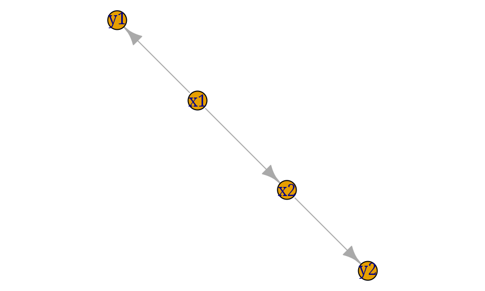
A network for $x$ can be constructed as:

u <- list(x1=yn, x2=yn)
x1 <- cpt(~x1, values=c(1, 3), levels=u)
x2 <- cpt(~x2|x1, values=c(3, 1, 1, 7), levels=u)
bn <- grain(compile_cpt(x1, x2))
querygrain(bn, simplify=TRUE)

##       yes     no
## x1 0.2500 0.7500
## x2 0.2812 0.7188

The augmentation of $y|x$ can go along these lines: The parameters describing $y|x$ are set to be:

s <- 2
mu <- c(mu1=2, mu2=5)
lambda <- c(lambda1=1, lambda2=5)

Suppose we observe $y_1 = y_1^*$. Then

$$\begin{align} p(x|y_1= y_1^*)\propto p(x_1)p(x_2|x_1) p(y_1=y_1^*|x_1) = p(x_1)p(x_2|x_1) L_1(x_1) \end{align}$$

where $L_1(x_1)$ denotes the likelihood. In a network setting this corresponds to changing $p(x_1)$ as $$\begin{align} p(x_1) \leftarrow p(x_1)L_1(x_1) \end{align}$$ and then carry on with propagation. This can be achieved in different ways.

The likelihood is:

y1_obs <- 14 # Observed value for y1_obs
lik1 <- dnorm(y1_obs, mean=mu, sd=s)
lik1

##       mu1       mu2 
## 3.038e-09 7.992e-06

One is by setting the likelihood as evidence. An alternative is to explicitly modify the CPT which specifies $p(x_1)$:

querygrain(bn, simplify=TRUE, exclude=FALSE)

##       yes     no
## x1 0.2500 0.7500
## x2 0.2812 0.7188

bn1 <- setEvidence(bn, evidence=list(x1=lik1))
querygrain(bn1, simplify=TRUE, exclude=FALSE)

##          yes     no
## x1 0.0001267 0.9999
## x2 0.1250792 0.8749

x1_upd <- getgrain(bn, "cptlist")$x1 * lik1
bn2 <- replace_cpt(bn, list(x1=x1_upd))
querygrain(bn2, simplify=TRUE) 

##          yes     no
## x1 0.0001267 0.9999
## x2 0.1250792 0.8749

A final remark: The conditional distribution of $y_1$ is normal, but the unconditional distribution is a mixture of normals. Likewise, the conditional distribution of $y_2$ is poisson, but the unconditional distribution is a mixture of two poisson distributions. Evidence on, say $y_1$ changes the belief in $x_1$ and $x_2$ and this in turn changes the distribution of $y_2$ (evidence changes the mixture weights.)

nsim <- 10000
xsim_marg <- simulate(bn, nsim, seed=2022)
xsim_cond <- simulate(bn1, nsim, seed=2022)
y2marg  <- rpois(n=nsim, lambda=lambda[xsim_marg$x2])
y2cond  <- rpois(n=nsim, lambda=lambda[xsim_cond$x2])
summary(y2marg)

##    Min. 1st Qu.  Median    Mean 3rd Qu.    Max. 
##    0.00    2.00    4.00    3.88    6.00   16.00

summary(y2cond)

##    Min. 1st Qu.  Median    Mean 3rd Qu.    Max. 
##    0.00    3.00    4.00    4.52    6.00   15.00

par(mfrow=c(1,2))
y2marg |> hist(prob=T, ylim=c(0, .4), breaks=20, main="marginal p(y2)")
y2cond |> hist(prob=T, ylim=c(0, .4), breaks=20, main="conditional p(y2|y1*)")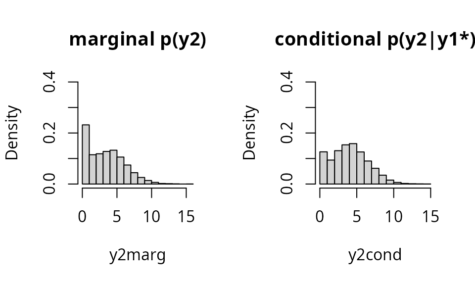

Brute force computations and why they fail

The gRain package makes computations as those outlined above in a very efficient way; please see the references. However, it is in this small example also possible to make the computations directly: We can construct the joint distribution (an array with $2^8=256$ entries) directly as:

joint <- tabProd(chest_cpt)
dim(joint)

## [1] 2 2 2 2 2 2 2 2

joint  |> as.data.frame.table() |> head()

##   xray smoke asia tub lung dysp bronc either      Freq
## 1  yes   yes  yes yes  yes  yes   yes    yes 1.323e-05
## 2   no   yes  yes yes  yes  yes   yes    yes 2.700e-07
## 3  yes    no  yes yes  yes  yes   yes    yes 6.615e-07
## 4   no    no  yes yes  yes  yes   yes    yes 1.350e-08
## 5  yes   yes   no yes  yes  yes   yes    yes 2.620e-04
## 6   no   yes   no yes  yes  yes   yes    yes 5.346e-06

This will clearly fail even moderate size problems: For example, a model with $80$ nodes each with $10$ levels will give a joint state space with $10^{80}$ states; that is about the number of atoms in the universe. Similarly, $265$ binary variables will result in a joint state space of about the same size. Yet, gRain has been used successfully in models with tens of thousand variables. The ``trick’’ in gRain is to make all computations without ever forming the joint distribution.

However, we can do all the computations by brute force methods as we will illustrate here:

Marginal distributions are

tabMarg(joint, "lung")

## lung
##   yes    no 
## 0.055 0.945

tabMarg(joint, "bronc")

## bronc
##  yes   no 
## 0.45 0.55

Conditioning on evidence can be done in different ways: The conditional density is a $6$–way slice of the original $8$–way joint distribution:

asia_dysp

## $asia
## [1] "yes"
## 
## $dysp
## [1] "yes"

cond1 <- tabSlice(joint, slice=asia_dysp)
cond1 <- cond1 / sum(cond1)
dim(cond1)

## [1] 2 2 2 2 2 2

tabMarg(cond1, "lung")

## lung
##     yes      no 
## 0.09953 0.90047

tabMarg(cond1, "bronc")

## bronc
##    yes     no 
## 0.8114 0.1886

Alternatively, multiply all entries not consistent by zero and all other entries by one and then marginalize:

cond2 <- tabSliceMult(joint, slice=asia_dysp)
cond2 <- cond2 / sum(cond2)
dim(cond2)

## [1] 2 2 2 2 2 2 2 2

tabMarg(cond2, "lung")

## lung
##     yes      no 
## 0.09953 0.90047

tabMarg(cond2, "bronc")

## bronc
##    yes     no 
## 0.8114 0.1886

Højsgaard, Søren. 2012. “Graphical Independence Networks with the gRain Package for R.” Journal of Statistical Software 46 (10): 1–26. http://www.jstatsoft.org/v46/i10/.

Højsgaard, Søren, David Edwards, and Steffen L. Lauritzen. 2012. Graphical Models with r. Springer.

Lauritzen, Steffen L., and David Spiegelhalter. 1988. “Local Computations with Probabilities on Graphical Structures and Their Application to Expert Systems.” J. Roy. Stat. Soc. Ser. B 50 (2): 157–224.